Note

Lec 2 Data¶

Types of Attributes¶

标称属性(nominal data)：代表某种类别、编码或者状态。比如头发颜色如黑色、棕色、黄色等。标称属性值不具有有意义的序且并不是定量的。众数是该属性的人中心趋势度量。均值和中位数都无意义。

不定量且无序，反应类别

序数属性(ordinal data)：值之间具有有意义的序(ranking)。相继值之间的差未知。比如标称属性 size 中的大、中、小，具有有意义的先后次序，但是无法描述大和中、中和小之间相差具体多少。序数属性也可以数值量的值域划分成有限有序类别，将数值属性离散化得到。序数属性的中心趋势度量可用众数和中位数表示，均值意义不大。

ranking

interval data: 用数字定量地描述变量程度上的差异。比如温度，20℃ 比 10℃ 高 10℃，和 30℃ 与 20℃ 之间的温差是一样的。这种情况下二者的差（interval）有意义的，而计数零点的选择是无关紧要的。选择不同的参考温度作为 0℃，那么同一温度会有不同的示数。但不影响两个温度之间的差。

ratio data:计数零点是有意义的，或者说不光变量之间的差有意义，而且变量本身就具有意义。比如长度，质量，在物理上有明确的定义：一米有多长，一千克有多少量。这样如果我们说 0.5 米我们就知道有多长。计数零点 0 米也是明确的，而不是可以任意选择的。

Example

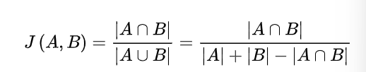
Jaccard 系数¶

Lec 3 Frequentist Data Analysis¶

Maximum Likelihood Estimation: $\hat{\theta}_{MLE}=\arg \max\limits_{\theta}P(D|\theta)$
对二项分布：

$$ \hat{p}=\arg\max\limits_{p}\mathbb{P}(X_1,\cdots,X_n;p) $$

$$ =\arg \max\limits_p {p^{n_h}(1-p)^{n-n_h} } $$

$$ =\arg\max\limits_p{n_h\log p+(n-n_h)\log(1-p)} $$

$$ => \frac{n_h}{\hat{p}}-\frac{n-n_h}{1-\hat{p}}=0 $$

$$ => \hat{p}=\frac{n_h}{n} $$

无偏性：多次重复后，频率趋近实际概率
指数分布 $$ f_X(x;\theta)= \theta e^{-\theta x},x\geq 0 $$

$$ \max\limits_{\theta}\prod\limits_{i=1}^n \theta e^{-\theta x_i}=\max\limits_\theta (n\log\theta-\theta\sum\limits_{i=1}^nx_i) $$

$$ \hat{\theta}_{ML}=\frac{n}{X_1+\cdots+X_n}=\frac{1}{\overline{X}} $$

正态分布：$\mu = \overline{x},\sigma^2=\frac{1}{n}\sum\limits_{i=1}^n(x_i-\mu)^2$
均匀分布：$\hat{\theta}=x_{(n)}=\max\{x_1,x_2,\cdots,x_n \}$
Poisson 分布：

\[ P(X=x)=\frac{\lambda^xe^{-\lambda}}{x!} \]

\[ \lambda = \frac{1}{n}\sum\limits\_{j=1}^nx_j \]

Lec 4 Bayesian Data Analysis¶

review：

$$ P(\theta| \mathcal{D})=\frac{P(\mathcal{D}|\theta)P(\theta)}{P(\mathcal{D})} \propto P(\mathcal{D}|\theta)P(\theta) $$

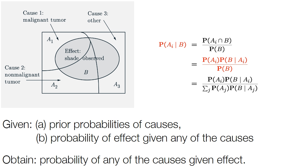
最大后验估计 MAP

\[ \theta_{MAP}=\arg\max\limits_{\theta}p_{model}(x;\theta)*p(\theta) \]

\[ =\arg\max\limits_{\theta}\prod\limits_{i=1}^Np_{model}(x^i;\theta)*p(\theta) \]

\[ =\arg\max\limits_{\theta}\sum\limits_{i=1}^N\log p_{model}(x^i;\theta)+\log p(\theta) \]

Lec 5 Testing¶

数据科学家需要帮助确保数据分析的结果不是错误的发现，即没有意义或可重复性

两个假设¶

我们想要反驳的陈述称为原假设或零假设(null hypothesis,$H_0$),原假设通常是结果仅由随机变化引起的陈述
一个随机变量$R$，称为检验统计量(test statistic) - $R$在$H_0$下的分布称为 null distribution - $R$的值从结果中得到，通常是数字

显著性检验¶

计算$R$为当前值或更极端情况的概率，此概率被称为检验统计量的p-value
如果 p 值足够小，则表示结果具有统计显著性
p 值的阈值被称为显著性水平(significance level,$\alpha$)，通常取 0.01 或 0.05
如果 p 值不够小，我们说我们无法拒绝原假设
$p-value = P(R|H_0)$

Neyman-Pearson 假设检验¶

明确指定备择假设(alternative hypothesis) $H_1$
显著性检验无法量化观察到的结果如何支持 $H_1$
定义一个替代分布，即当$H_1$为真时检验统计量的分布
我们为检验统计量$R$定义一个临界区域(critical region)，如果$R$落在此区域中，我们拒绝$H_0$。
若$H_0$被拒绝，我们可能会也可能不会接受$H_1$
显著性水平$\alpha$是在$H_0$下临界区域概率
Type Ⅰ Error ($\alpha$)
等于$H_0$下临界区域概率，即显著性水平
$\alpha=P(R\in Crtical\ Region | H_0)$
Type Ⅱ Error ($\beta$)
当备择假设为真时，错误地将结果称为不显著
$\beta=P(R\notin Critical\ Region| H_1)$
Power(功效)：即 $H_1$ 下临界区域的概率，即 $1−β$。
Power 表明一个测试正确拒绝原假设的正确性
低功耗意味着许多实际显示所需模式或现象的结果将不被视为重要结果，因此会被遗漏
因此，如果测试的功效较低，那么忽略临界区域之外的结果可能不合适。

Binary Hypothesis Testing¶

null hypothesis $H_0:X~ p_X(x;H_0)$
alternative hypothesis $H_1: X~p_X(x;H_1)$

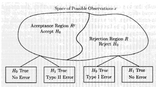
Type Ⅰ Error：错误的拒绝，错误的预警 $\alpha(R)=P(X\in R;H_0)$
Type Ⅱ Error：错误的接受，遗漏，$H_0$ false, but accepted

Bayesian Hypothesis Testing¶

$\Theta$在$\{\theta_1,\cdots,\theta_m \}$m 个值中选一个
$H_i\equiv event\{\Theta = \theta_i \}$
假设检验：给定观测值$x$，从$H_1\cdots H_m$中选一个假设
MAP Rule：选择后验概率最大的假设，即选择$H_i$若$P(\Theta=\theta_i|X=x)=p_{\Theta|X}(\theta_i|x)$最大
即$p_{\Theta}(\theta_i)p_{X|\Theta}(x|\theta_i)$($X$离散)或$p_{\Theta}(\theta_i)f_{X|\Theta}(x|\theta_i)$($X$连续)最大

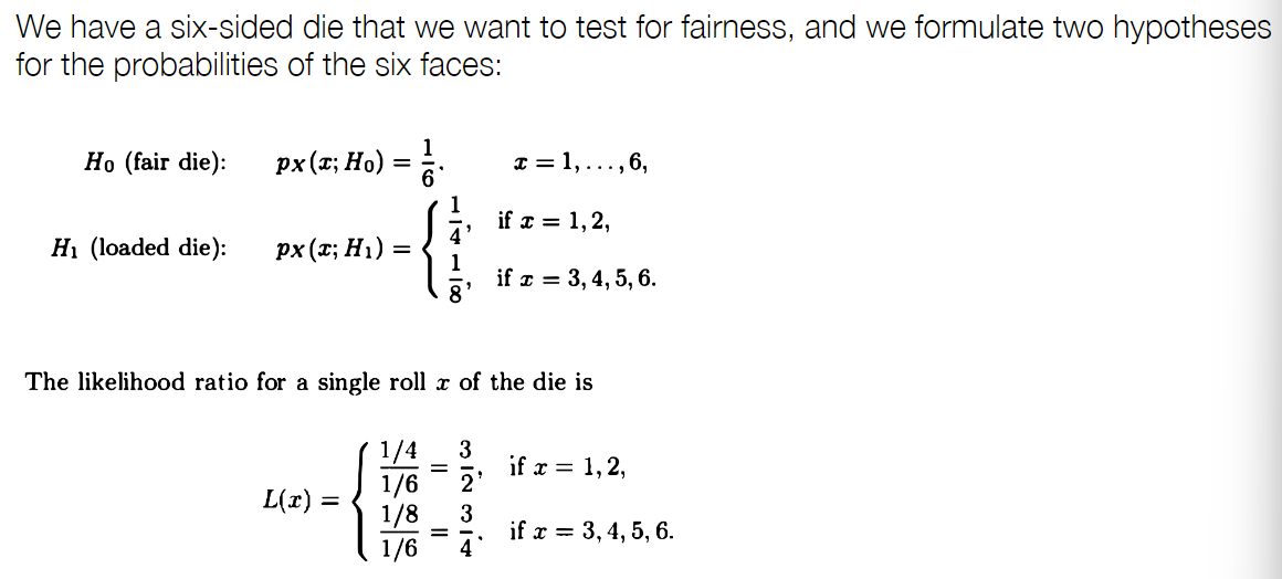
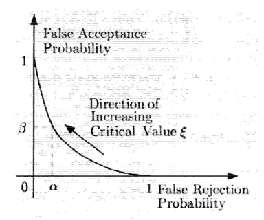
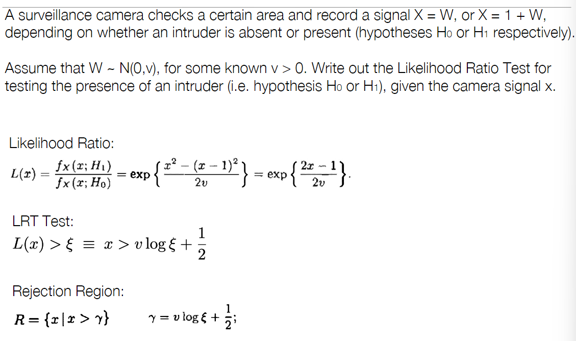
Likelihood Ratio Test (LRT)¶

选择$H_1$若

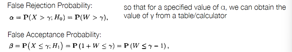
\[ L(x)=\frac{P(X=x;H_1)}{P(X=x;H_0)}>\xi \ (discrete\ case) \]

\[ L(x)=\frac{f_X(x;H_1)}{f_X(x;H_0)}>\xi \ (continuous\ case) \]

阈值$\xi$ 权衡两种错误，选择$\xi$使得$P(reject\ H_0;H_0)=\alpha$

Example

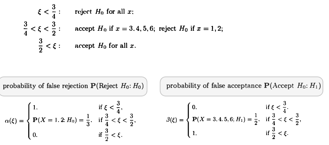
Summary
Start with a target value a for the false rejection probability
选择$\xi$，使得$P(L(X)>\xi;H_0)=\alpha$
拒绝$H_0$，若$L(x)>\xi$

Example

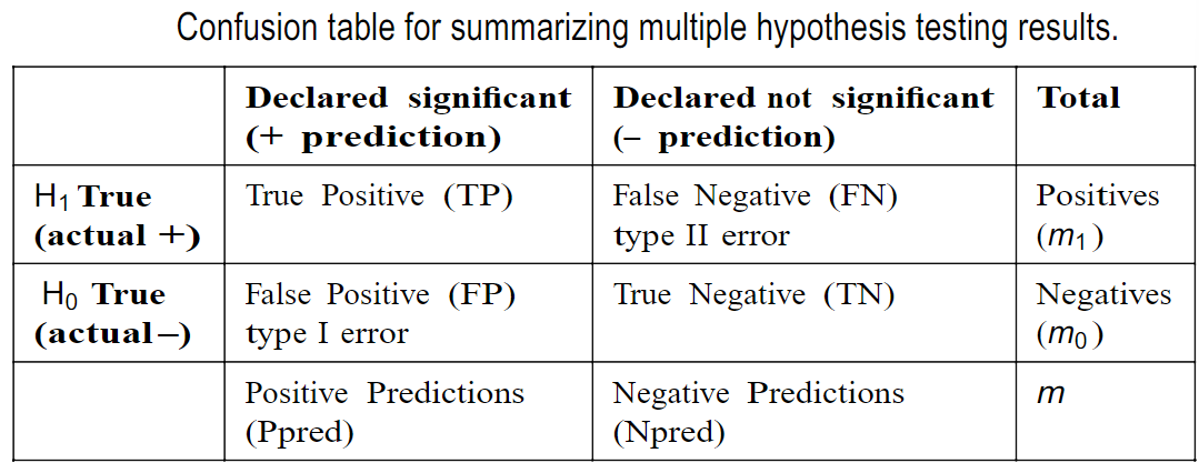
Multiple Hypothesis Testing¶

We assume the results fall into two classes, + and -, which, follow the alternative and null hypotheses, respectively
重点通常放在误报（FP）的数量上，即属于 null 分布 (- 类) 但声明为显著性 (+ 类)的结果。

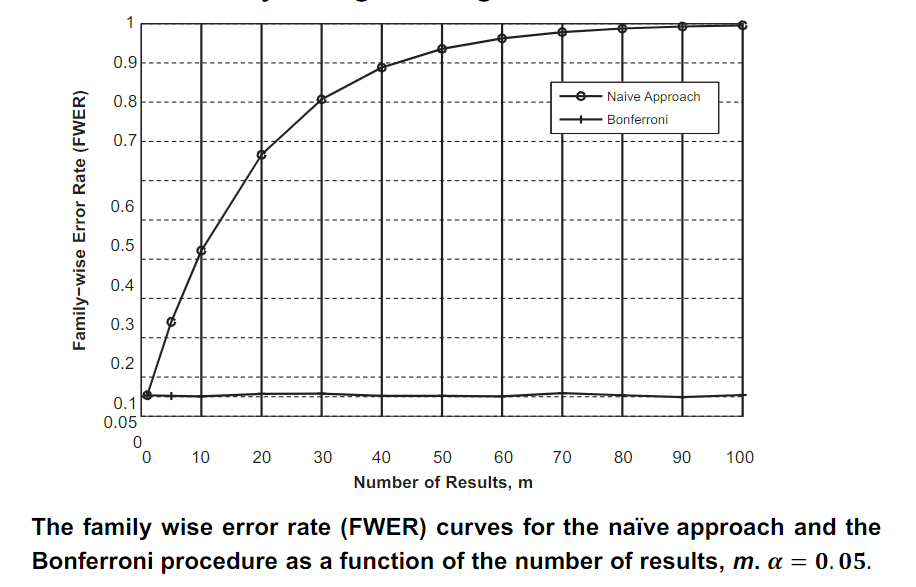
Family-wise Error Rate¶

$FWER = P(FP > 0)$
假设显著性水平是 0.05
则一次测试没有错误的概率是 1-0.05=0.95
m 次测试没有错误是$0.95^m$
则$FWER=P(FP>0)=1-0.95^m$
若$m=10,FWER=0.60$

Bonferroni Procedure¶

FWER 的目标是确保$FWER<\alpha$，其中$\alpha$通常取 0.05
Bonferroni Procedure
$m$ results are to be tested
Require $FWER < α$
set the significance level, $\alpha^*$ for every test to be $\alpha^*=\alpha/m$
If $m = 10$ and $\alpha= 0.05$ then $\alpha^* = 0.05/10=0.005$
Example: Bonferroni versus Naïve approach
朴素的方法是在不调整显著性水平的情况下评估每个结果的统计显著性。

Lec 6 Unsupervised Learning¶

Background¶

关于相似性¶

相似性的真正含义是一个哲学问题。我们将采取一种更务实的方法——从向量之间的距离（而不是相似性）或随机变量之间的相关性的角度来思考。

距离指标¶

given $x=(x_1,x_2,\cdots,x_p), y=(y_1,y_2,\cdots,y_p)$

Euclidean 距离: $d(x,y)=\sqrt{\sum\limits_{i=1}^p|x_i-y_i|^2}$

Manhattan 距离: $d(x,y)=\sum\limits_{i=1}^p|x_i-y_i|$

Sup-distance: $d(x,y)=\max\limits_{1\leq i\leq p}|x_i-y_i|$

Pearson 相关系数:

\[ \rho(x,y)=\frac{\sum\limits_{i=1}^p(x_i-\overline{x})(y_i-\overline{y})}{\sqrt{\sum\limits_{i=1}^p(x_i-\overline{x})^2\times\sum\limits_{i=1}^p(y_i-\overline{y})^2}} \]

Clustering Algorithms¶

Hierarchical algorithms 分层¶

single-linkage

average-linkage

complete-linkage

centroid-based

Bottom-Up Agglomerative Clustering
Starts with each object in a separate cluster, and repeat:
- Joins the most similar pair of clusters,
- Update the similarity of the new cluster to others until there is only one cluster.
Greedy – less accurate but simple to implement
Top-Down divisive
Starts with all the data in a single cluster, and repeat:
- Split each cluster into two using a partition algorithm until each object is a separate cluster.
More accurate but complex to implement
对于 Agglomerative Clustering：basic 算法直接明了

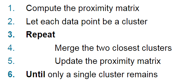
关键在于计算两个类之间的邻近矩阵

Cluster Similarity¶

MIN(single link): 两个聚类的相似性基于不同聚类中两个最相似（最接近）的点，也就是由一对点决定
优势：可以处理非椭圆形(non-eliptical shapes)，对噪声和异常值敏感
MAX(complete link): 两个聚类的相似性基于不同聚类中两个最不相似（最远）的点，由两个聚类中的所有点对确定
优势：不易受到噪点和异常值的影响
局限性：倾向于 break 大型聚类

Group Average: 两个聚类的邻近性是两个聚类中点之间成对接近的平均值。

\[ proximity(Cluster_i,Cluster_j)=\frac{\sum\limits_{p_i\in Cluster_i,p_j\in Cluster_j}proximity(p_i,p_j)}{|Cluster_i|\times|Cluster_j|} \]

需要使用平均连接来实现可扩展性，因为总邻近性有利于大型集群
single link 和 complete link 之间的折中
Single vs. Complete Linkage
single-linkage:允许各向异性和非凸形
complete-linkage:假定各向同性凸形

计算复杂度¶

All hierarchical clustering methods need to compute similarity of all pairs of $n$ individual instances which is $O(n^2)$
At each iteration,
Find largest of the set of similarities $O(n^2)$
Update similarity between merged cluster and other clusters $O(n)$
Maximum no. of iterations $O(n)$
So we get time complexity of $O(n^3)$
could be reduced with more complicated data structures such as heaps which however come with greater storage complexity

Partitioning Algorithms¶

Given: a set of $n$ objects and number $K$, construct a partition of $n$ objects into a set of $K$ clusters

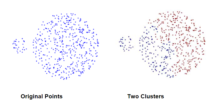
K-Means¶

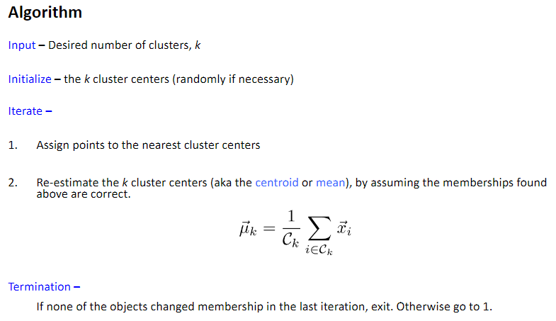
每个聚类都与一个质心（中心点）相关联
每个点都分配给具有最接近质心的聚类

计算复杂度¶

At each iteration,
Computing distance between each of the $n$ objects and the $K$ cluster centers is $O(Kn)$.
Computing cluster centers: Each object gets added once to some cluster: $O(n)$.
Assume these two steps are each done once for l iterations: $O(lKn)$.

Seed Choice¶

聚类结果对初始种子选择很敏感
一些种子可能导致收敛率差，或收敛到次优聚类
使用启发式方法选择好的种子（例如，与任何现有均值最不相似的对象）
k-means ++ algorithm of Arthur and Vassilvitskii
key idea: 选择相距较远的中心
选择一个点作为聚类中心的概率与到目前为止选择的与最近中心的距离成正比
尝试多个起点非常重要
使用其他方法的结果进行初始化

Other Issues¶

簇的形状：假设各向同性、等方差、凸聚类
对异常值敏感：使用 K-medoids
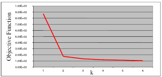
聚类数目
目标函数: $\sum\limits_{j=1}^m ||\mu_C(j)-x_j||^2$
找目标函数中的 knee

Lec 7.1 Unsupervised Learning Contd.¶

Graph-based Clustering¶

Graph-Based clustering uses the proximity graph

Problem: too many edges

Sparsification(稀疏化)¶

数据量需要被大量减少
稀疏化可以去邻接矩阵中 99%以上的条目
耗时减少了
可处理问题规模上升了
稀疏化后聚类效果可能更好
稀疏化使得点与其最近似点保持连接而断开和其他 less similar 点的连接
The nearest neighbors of a point tend to belong to the same class as the point itself.
降低了噪声和异常值的影响

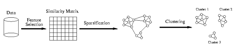
SNN Clustering¶

计算相似度矩阵：这对应于具有节点和边的数据点的相似性图，其权重是数据点之间的相似性
通过仅保留 k 个最相似的邻居来稀疏化相似度矩阵这相当于只保留相似性图的 k 个最强链接
Construct the shared nearest neighbor graph from the sparsified similarity matrix.

此时，我们可以应用相似性阈值并找到 connected components 来获得聚类

求每个点的 SNN 密度 - 使用用户指定的参数 Eps 查找与每个点的 SNN 相似度为 Eps 或更大的数点。这是该点的 SNN 密度

Lec 7.2 Anomaly Detection 异常检测¶

Chanllenges
异常值数量
方法是无监督的，validation 将会很困难
Finding needle in a haystack
Working assumption: 正常值比异常值多

General Steps¶

Build a profile of the normal behavior
Profile can be patterns or summary statistics for the overall population
Use the normal profile to detect anomalies
Anomalies are observations whose characteristics differ significantly from the normal profile

Distance-based Approaches¶

数据用特征向量表示
三个主要方法：Nearest-neighbor based, density based, clustering based

Nearest-Neighbor Based Approach¶

define 异常值方法：

距离$D$内少于$p$个点
到第$k$个最近点的距离最大的前$n$个点
与前$k$个最近点距离的平均值最大的前$n$个点

Clustering-Based¶

Basic idea:
Cluster the data into groups of different density
Choose points in small cluster as candidate outliers
Compute the distance between candidate points and non-candidate clusters.
- If candidate points are far from all other non-candidate points, they are outliers

Lec 7.3 SVD/PCA, Symbols to Meaning¶

Symbols to Meaning¶

An important goal in AI is to go from these low-level features/symbols, which we observe, to meaning, which we do not see/observe

我们观察到的：构成数据的“原始”特征和符号（例如文本文档中的单词）
我们所说的“意义”是指原始特征背后的概念
这些概念可以用来“解释”数据（例如，如果你在字典里看，任何单词的含义都是用概念来解释的）
这些概念从未被直接观察到

Document Data¶

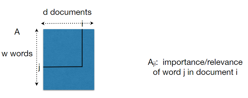
对一组文档，我们可以将其收集为如图所示的数据矩阵，其中行表示 words(features), 列表示 documents(samples)
$A_{ji}=t_{ji}\times g_j\times s_i$
$t_{ji}$: word $j$ 在文档 $i$ 中出现次数
$g_j$: 在整个文档集合中 word $j$ 的重要性
- 例如： $\log\frac{d}{d_j}$， $d_j$是出现 word $j$ 的文档数量
$s_i$: 用于归一化，$s_i=\frac{1}{\sqrt{\sum_{j=1}^w(t_{ji}g_j)^2}}$
通过以上步骤，A 的列被归一化了，也就是$||a_i||_2=1$

Which document is most similar?¶

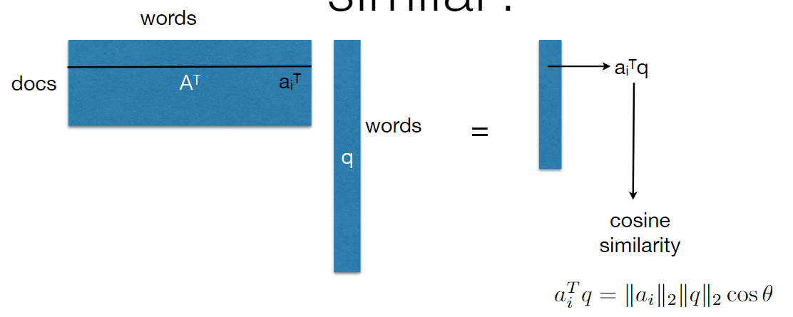
$q$ 表示 query
如果一个文档不包含要找的单词，相似度就是 0

仅使用 syntax 的注意事项¶

computational：即使对特征进行剪枝后，单词数量也会是数万级别
Not as intelligent
不能判断同义词，e.g. searching for MRI would miss “Magnetic Resonance Imaging”
不能判断多义词，e.g. “mining” could refer to “data mining” or “coal mining”
为了提取文档的概念，我们可以使用潜在语义分析 Latent Semantic Analysis (LSA)

Latent Semantic Analysis¶

PCA¶

SVD 奇异值分解

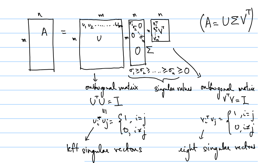
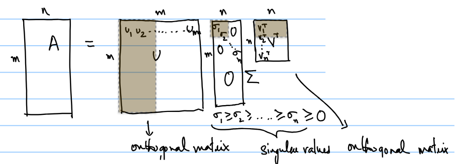
PCA：use only the top k columns of U and V

LSA¶

Obtain PCA approximation of document data matrix
Use principal components as “concepts”
Many singular vectors i.e. concepts are required to approximate document data matrix well (k ~ 1000)
Does not work well to capture concepts from short documents e.g. queries (and hence no search engine uses this)

Beyond LSA¶

非负矩阵分解（NMF）：将权重约束为非负

假设我们约束：
概念是单词的（多项式）分布
文档是概念的（多项式）分布
Probabilistic latent semantic analysis
- Latent Dirichlet Allocation (LDA) (Blei et al, 2003); also known as a “topic model” very closely related

Lec 8 Supervised Learning¶

Optimal Classification¶

贝叶斯分类器: $f^*=\arg\min\limits_f P(f(X)\neq Y)$

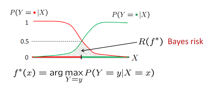
Even the optimal classifier makes mistakes
最佳分类器取决于未知分布

\[ f^*(x)=\arg\max\limits_{Y=y}P(Y=y|X=x) \\ =\arg\max\limits_{Y=y}P(X=x|Y=y)P(Y=y) \]

对贝叶斯分类器，若各类之间独立 $P(X_1\dots X_d|Y)=\prod\limits_{i=1}^d P(X_i|Y)$

则 $f_{NB}(x)=\arg\max\limits_y P(x_1,\dots,x_d|y)P(y)=\arg\max\limits_y\prod\limits_{i=1}^d P(x_i|y)P(y)$

有条件的独立性
X is conditionally independent of Y given Z: probability distribution governing X is independent of the value of Y, given the value of Z

\[(\forall x,y,z)P(X=x|Y=y,Z=z)=P(X=x|Z=z)\]

即$P(X,Y|Z)=P(X|Z)P(Y|Z)$

Logistic Regression¶

\[P(Y=1|X)=\frac{1}{1+\exp(w_0+\sum_i w_iX_I)}\]

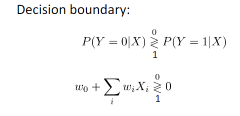
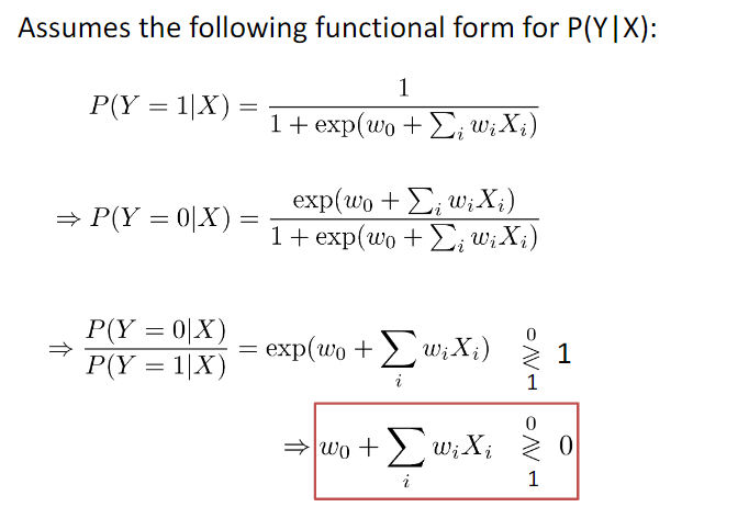
线性分类器

Lec 9 Supervised Learning II¶

TODO

Lec 10 Supervised Learning III¶

Classification¶

Decision Tree¶

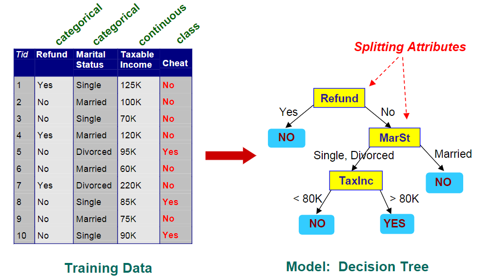
Hunt's Algorithm¶

$D_t$为训练记录集合，$t$为节点

$D_t$所有记录属于类$y_t$，t 为叶节点，类型即为$y_t$
$D_t$为空，t 类型为默认类型$y_d$(default)
$D_t$中的记录属于不止一类，则使用 attribute test 将数据分成更小的子集

递归调用以上过程

test condition¶

Greedy strategy: split the record based on an attribute test that optimizes certain criterion
How to specify test condition
depends on attribute types: nominal, ordinal, continuous
depends on number of ways to split:
- 2-way split: divides values into two subsets, need to find optimal partitioning
- multi-way split: use as many partitions as distinct values
For continuous attributes
Binary decision: $A<v$ or $A\geq v$
How to determine best split
Greedy: 优先考虑具有均匀类分布的节点
node impurity:

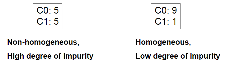
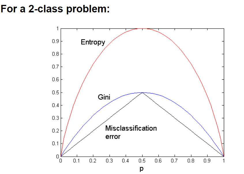
$GINI(t)=1-\sum\limits_j[p(j|t)]^2$，其中$p(j|t)$是节点 t 处类 j 的相对频率
- 最大值为$1-1/n_c$当所有记录均匀分布时取到
- 最小值为 0，当所有记录都属于同一类
- 分裂成 k 个部分时，$GINI_{split}=\sum\limits_{i=1}^k\frac{n_i}{n}GINI(i)$
$Entropy(t)=-\sum\limits_jp(j|t)\log p(j|t)$
- 类似最大值$\log n_c$均匀分布取到，最小值 0 同一类取到
- 信息增益: $GAIN_{split}=Entropy(p)-(\sum\limits_{i=1}^k\frac{n_i}{n}Entropy(i))$
- 更进一步，$GainRATIO_{split}=\frac{GAIN_{split}}{SplitINFO}$，其中$SplitINFO=-\sum\limits_{i=1}^k\frac{n_i}{n}\log \frac{n_i}{n}$
Classification error: $Error(t)=1-\max\limits_i P(i|t)$
- 最大值为$1-1/n_c$当所有记录均匀分布时取到
- 最小值为 0，当所有记录都属于同一类

Stopping Criteria for Tree Induction¶

当所有记录都属于同一个类时停止展开节点
当所有记录具有相似的属性值时停止展开节点
提前终止

Decision Tree Based Classification¶

Advantages
构建成本低
分类未知数据速度快
易于对小规模树进行解释
对许多简单数据集，准确率可以与其他分类方式相当

Note

Lec 2 Data¶

Types of Attributes¶

Jaccard 系数¶

Lec 3 Frequentist Data Analysis¶

Lec 4 Bayesian Data Analysis¶

Lec 5 Testing¶

两个假设¶

显著性检验¶

Neyman-Pearson 假设检验¶

Binary Hypothesis Testing¶

Bayesian Hypothesis Testing¶

Likelihood Ratio Test (LRT)¶

Multiple Hypothesis Testing¶

Family-wise Error Rate¶

Bonferroni Procedure¶

Lec 6 Unsupervised Learning¶

Background¶

关于相似性¶

距离指标¶

Clustering Algorithms¶

Hierarchical algorithms 分层¶

Cluster Similarity¶

计算复杂度¶

Partitioning Algorithms¶

K-Means¶

计算复杂度¶

Seed Choice¶

Other Issues¶

Lec 7.1 Unsupervised Learning Contd.¶

Graph-based Clustering¶

Sparsification(稀疏化)¶

SNN Clustering¶

Lec 7.2 Anomaly Detection 异常检测¶

General Steps¶

Distance-based Approaches¶

Nearest-Neighbor Based Approach¶

Clustering-Based¶

Lec 7.3 SVD/PCA, Symbols to Meaning¶

Symbols to Meaning¶

Document Data¶

Which document is most similar?¶

仅使用 syntax 的注意事项¶

Latent Semantic Analysis¶

PCA¶

LSA¶

Beyond LSA¶

Lec 8 Supervised Learning¶

Optimal Classification¶

Logistic Regression¶

Lec 9 Supervised Learning II¶

Lec 10 Supervised Learning III¶

Classification¶

Decision Tree¶

Hunt's Algorithm¶

test condition¶

Stopping Criteria for Tree Induction¶

Decision Tree Based Classification¶

评论