8 Bayesian Decision Theory¶

Prior¶

A priori (prior) probability of the state of nature
- Random variable (State of nature is unpredictable)
- Reflects our prior knowledge about how likely we are to observe a sea bass or salmon
- The catch of salmon and sea bass is equiprobable
  - $P(w_1)=P(w_2)$ uniform priors
  - $P(w_1)+P(w_2)=1$ exclusivity and exhaustively
只有先验时：选择概率较大的那一个为结果，错误率为概率小的另一个

Likelihood¶

假设我们知道要分类物体的某个特征，比如鱼表面的颜色，这时候$p(x|w_1)$就表示种类是1的时候有x特征的概率，这个概率就是likelihood
maximum likelihood decision: assign input pattern $x$ to class $w_1$ if $p(x|w_1)>p(x|w_2)$

Posterior¶

Posterior = (Likelihood x Prior) / Evidence $p(w_i|x)=\dfrac{p(x|w_i)p(w_i)}{p(x)}$
- Evidence $p(x)$ can be viewed as a scale factor that guarantees that the posterior probabilities sum to 1

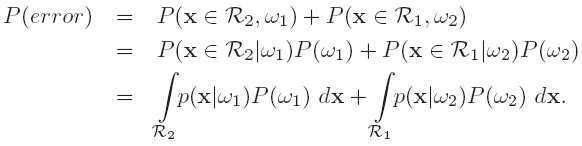
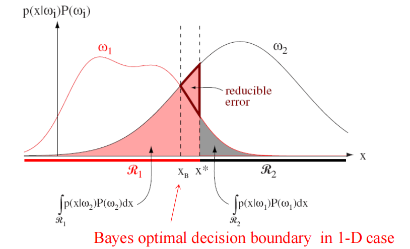
Optimal Bayes Decision Rule¶

Generalization¶

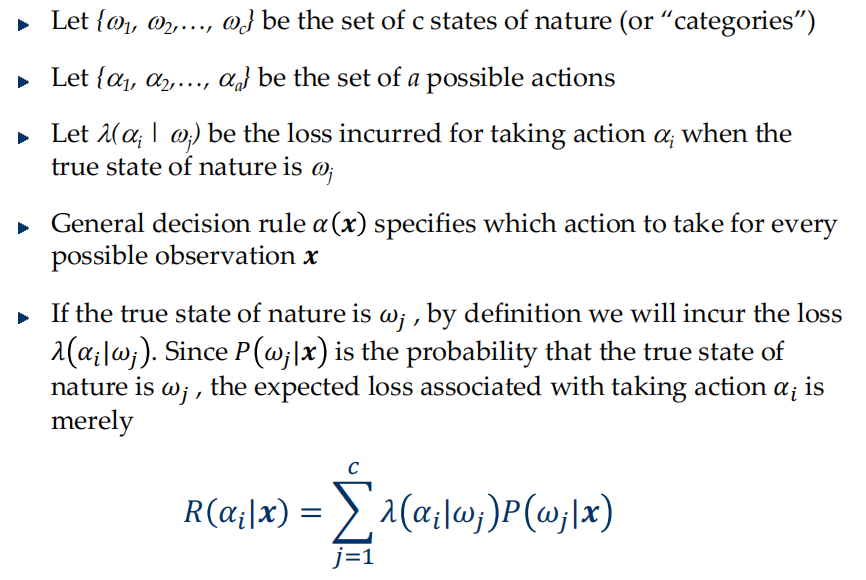
overall risk: $R=\int R(\alpha_i|x)p(x)dx$
- Bayes risk = best performance that can be achieved
conditional risk: $R(\alpha_i|x)=\sum\limits_{j=1}^c\lambda(\alpha_i|w_j)P(w_j|x)$
- 选择使$R(\alpha_i|x)$最小的action
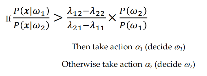
two-category classification
- If the likelihood ratio exceeds a threshold value that is independent of the input pattern x, we can take optimal actions

Minimum-Error-Rate Classification
- actions are decisions on classes
- seek a decision rule that minimizes the probability of error or the error rate
- Zero-one (0-1) loss function: no loss for correct decision and a unit loss for any error
- 这时候conditional risk $R(\alpha_i|x)=1-P(w_i|x)$，所以最小化risk等于最大化后验概率
- 在前面我们选择后验概率最大的作为选择，我们可以进一步抽象，把选择哪一类的称为discriminant functions $g_i(x)$
- $P(w_1|x) $ -> $p(x|w_1)P(w_1)$ -> $\ln p(x|w_1)+\ln P(w_1)$ -> $g(x)=P(w_1|x)-P(w_2|x)$ -> $g(x)=\ln\dfrac{p(x|w_1)}{p(x|w_2)}+\ln\dfrac{P(w_1)}{P(w_2)}$
MLE: Best parameters are obtained by maximizing the probability of obtaining the samples observed
Log-likelihood

\[ l(\theta)=\ln p(D|\theta) \ \ \ \ p(D|\theta)=\prod^n_{k=1}p(x_k|\theta)\newline l(\theta)=\sum_{k=1}^n\ln p(x_k|\theta)\newline \theta^*=arg\max_{\theta} l(\theta) \]
- set of necessary conditions for an optimum is $\nabla_{\theta}l=0$
Bayesian learning
- goal: estimating $p(x|w_i), p(x|D_i), p(x|w_i, D_i)$
- Use a set D of samples drawn independently according to the fixed but unknown probability distribution $p(x)$ to determine 已知分布，但不知道具体参数，因此相当于$p(x|\theta)$已知
General Theory
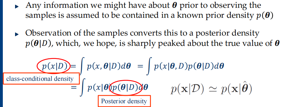
- The form of $p(x|\theta)$ is assumed known, but the value of $\theta$ is not known exactly
- Our knowledge about $\theta$ is assumed to be contained in a known prior density $p(\theta)$
- The rest of our knowledge about $\theta$ is contained in a set D of n random variables $x_1, x_2, \dots, x_n$ that follows $p(x)$
- Compute the posterior $p(\theta|D)$ , then estimate the class conditional density $p(x|D)$
朴素贝叶斯分类器：假设所有属性相互独立
- 优点
  - 对离群的噪声点鲁棒
  - 对缺失值，直接忽略
  - 对无关属性鲁棒
- 缺点
  - 假设在现实中很难成立
  - 需要拉普拉斯平滑
How to estimate probabilities from data? For continuous attributes
- discretize the range into bins: one ordinal attribute per bin
- two-way split: choose only one of the two splits as new attribute
- probability density estimation: 假设属性服从正态分布，用数据估计参数，再用参数估计概率
Laplace Smoothing 避免出现零概率使得相乘后为0

\[ \begin{aligned} P(x_{i}|\omega_{k})&=\frac{|x_{ik}|+1}{N_{\omega_{k}}+K}\newline P(x_{i}|\omega_{k})&=\frac{|x_{ik}|+\alpha}{N_{\omega_{k}}+\alpha K} \end{aligned} \]

8 Bayesian Decision Theory¶

Prior¶

Likelihood¶

Posterior¶

Optimal Bayes Decision Rule¶

Generalization¶

评论