6 Decision Tree

1. classifiers for instances represented as features vectors
2. nodes are tests for feature values

3. leaves specify the labels

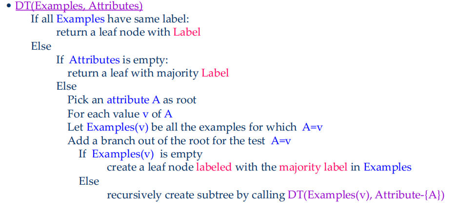
4. basic decision tree learning algorithm

5. Finding the minimal decision tree consistent with the data is NP-hard

6. Entropy: \(Entropy(S)=-P_{+}\log P_{+}-P_{-}\log P_{-}\)

   • all the examples belong to the same category, \(Entropy=0\)
   • the examples are equally mixed \((0.5,0.5), Entropy=1\)
   • in general, \(Entropy(S)=-\sum\limits_{i=1}^cP_i\log P_i\)

7. information gain: \(Gain(S,a)=Entropy(S)-\sum\limits_{v\in values(a)}\dfrac{|S_v|}{|S|}Entropy(S_v)\),where \(S_v\) is the subset of \(S\) for which attribute \(a\) has value \(v\)

   • partitions of low entropy lead to high gain

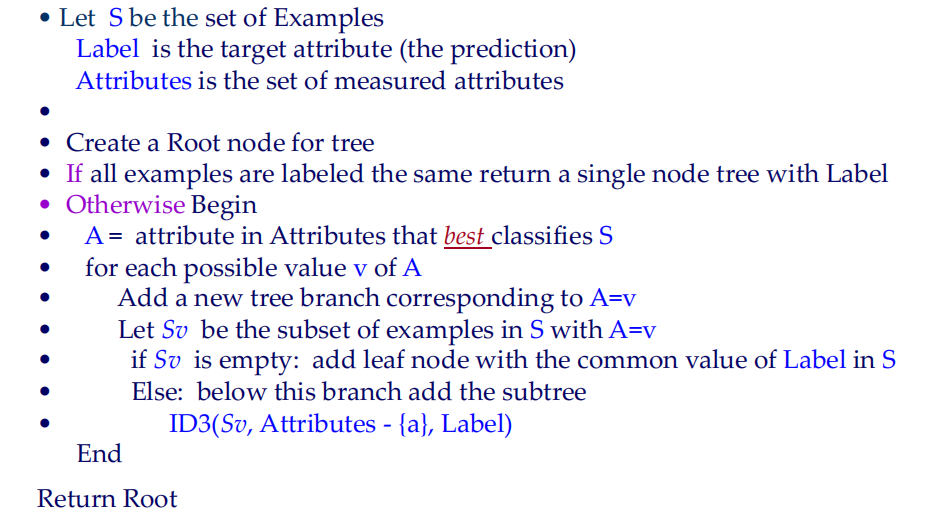
8. ID3(Examples, Attributes, Label)

   

9. Avoid overfitting

   • Prepruning: 在决策树生成过程中，对每个结点在划分前先进行估计，若当前结点的划分不能带来决策树泛化性能提升，则停止划分。
     • 泛化性能：将数据集划分一部分作为验证集，比较划分前后验证集的正确率
   • Postpruning：先生成一棵完整的决策树，自底向上考察非叶结点，若该结点对应的子树替换为叶结点能带来决策树泛化性能提升，则替换。

10. ID3: only for classification, the features must be discrete

11. CART(Classification and Regression Trees)

    • pick feature \(x^{(j)}\) as splitting variable and \(s\) as the splitting point, we have two regions: \(\mathcal{R}_1(j,s)=\{x|x^{(j)}\leq s\},\mathcal{R}_2(j,s)=\{x|x^{(j)}>s\}\)

    • calculate

      \[ \min_{j,s}[\min_{c_1}\sum_{x_i\in\mathcal{R}_1(j,s)}(y_i-c_1)^2+\min_{c_2}\sum_{x_i\in\mathcal{R}_2(j,s)}(y_i-c_2)^2] \]

    • find the best \((j,s)\) pair and then have two regions

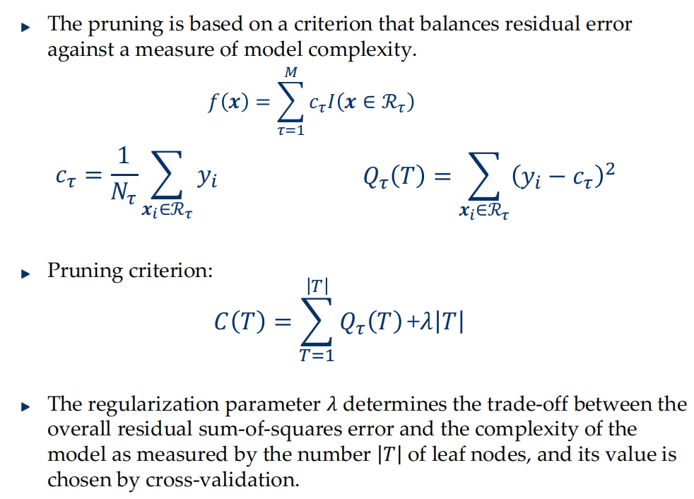
    • finally we have \(M\) regions, and the tree can be represented as \(f(x)=\sum\limits_{\tau=1}^M c_\tau I(x\in\mathcal{R}_\tau)\)
    • prune
    

    • for classification, just use Entropy or Gini index instead of residual sum-of-squares

      • the entropy: \(Q_\tau(T)=-\sum\limits_{k=1}^Kp_{\tau k}\log p_{\tau k}\)
      • the Gini index: \(Q_\tau(T)=\sum\limits_{k=1}^K p_{\tau k}(1-p_{\tau k})=1-\sum p_{\tau k}^2\)

评论