4 Linear Classifier

1. Binary classifier to multi-class classifier

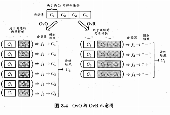
   • one vs. one: 将类别两两配对，产生\(N(N-1)/2\)个二分类任务，训练这些分类器。预测时将样本提交给所有分类器，结果中被预测的最多的即为最终分类结果
   • one vs. rest：每次将一个类作为正例，其余反例，训练N个分类器，预测时将输出正例的视为预测结果。
   
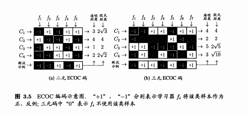
   • Error Correcting Output Codes(ECOC)，属于MvM
     • 编码：对N个类别做M次划分,每次划分将一部分类别划为正类，一部分划为反类,从而形成一个二分类训练集;这样一共产生M个训练集,可训练出M个分类器
     • 解码：M个分类器分别对测试样本进行预测，这些预测标记组成一个编码.将这个预测编码与每个类别各自的编码进行比较,返回其中距离最小的类别作为最终预测结果
     • 编码越长，纠错能力越强

2. sigmoid function: \(\sigma(t)=\dfrac{1}{1+e^{-t}}, \sigma:R\rightarrow(0,1)\)

3. Maximum likelihood estimation for logistic regression:

   \[ P(D)=\prod_{i\in I}\sigma(y_{i}\boldsymbol{a}^{T}\boldsymbol{x}_{i})\newline l\big(P(D)\big)=\sum_{i\in I}\log\bigl(\sigma(y_{i}\boldsymbol{a}^{T}\boldsymbol{x}_{i})\big)=-\sum_{i\in I}\log\bigl(1+e^{-y_{i}\boldsymbol{a}^{T}\boldsymbol{x}_{i}}\bigr) \newline E(\boldsymbol{a})=\sum_{i\in I}\log\left(1+e^{-y_i\boldsymbol{a}^T\boldsymbol{x}_i}\right) \]

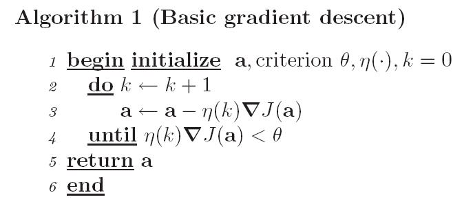
4. gradient descent algorithm

   

5. minimize a differentiable function:

   \[ E(a+\Delta a)=E(a)+E'(a)\Delta a+E''(a)\frac{\Delta a^2}{2!}+E'''(a)\frac{\Delta a^3}{3!}+\cdots \]

   • linear approximation: \(\Delta a=-\eta E^{\prime}(a)\)

   • quadratic approximation:

     • Newton's Method: Choose \(\Delta a\) that \(E^{\prime }( a) \Delta a+ E^{\prime \prime }( a) \frac {\Delta a^{2}}{2! }\)is minimum

     $$ \begin{aligned} E^{\prime}(a)+&E^{\prime\prime}(a)\Delta a=0\quad\newline \Delta\boldsymbol{a}=&-\eta[\mathbf{H}E(\boldsymbol{a})]^{-1}E^{\prime}(\boldsymbol{a}) \newline
     \Delta a=&-\frac{E'(a)}{E''(a)} \end{aligned} $$

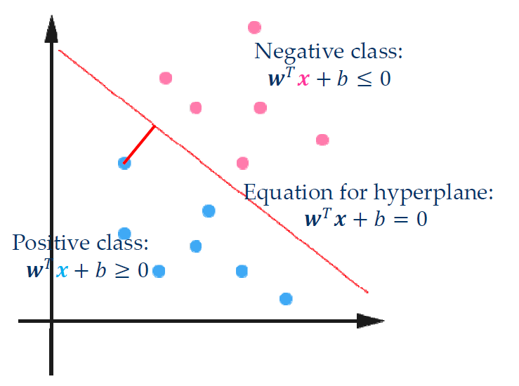
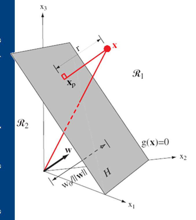
6. Support Vector Machine: hyperplane, decision surface

   

   • 对离群点敏感度

   • geometrical margin几何距离: \(\gamma=y\dfrac{w^Tx+b}{\|w\|}\) y保证非负

   

   • If the hyperplane moves a little, points with small \(\gamma\) will be affected, but points with large \(\gamma\) won’t

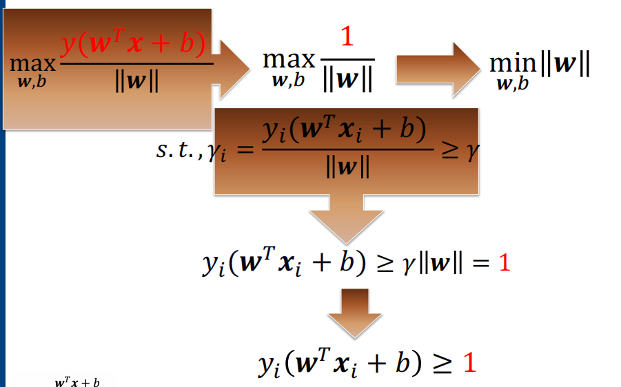
   • Maximum Margin Classifier: find the hyperplane with the largest margin, maximize the confidence of classifying the dataset

   • We know \(y(w^Tx+b)\) can be made arbitrarily large without changing the hyperplane, so we simply fix it at \(y(w^Tx+b)=1\)

   • so \(\min\limits_{w,b}\dfrac{1}{2}||w||^2\) and \(y_i(w^Tx_i+b)\geq1\)
   

   • weakness: When an outlier appear, the optimal hyperplane may be pushed far away from its original /correct place. The resultant margin will also be smaller than before.

   • slack variables: Assign a slack variable \(\xi\) to each data point. That means we allow the point to deviate from the correct margin by a distance of \(\xi\) (Actually \(\|w\|\xi\) when considering geometrical margin).

   • Unconstrained Optimization Problem of SVM

     \[ \min_{w,b}\frac12\|w\|^2+C\sum_{i=1}^n\xi_i\newline y(\boldsymbol{w}^T\boldsymbol{x}_i+b)\geq1-\xi_i\newline \xi_i\geq0 \newline \xi_{i}\geq1-y(w^{T}x_{i}+b)\quad\xi_{i}=\max[1-y(w^{T}x_{i}+b),0]\newline \min_{w,b}\left\{\sum^{n}_{i=1}\max[1-y(w^{T}x_{i}+b),0]+\frac{1}{2C}\|w\|^{2}\right\} \newline \ell(f)=\max[1-yf,0]\ \ \ \text{Hingeloss} \]

7. A General formulation of classifiers

   

   • Square loss: \(\ell(f)=(1-yf)^2\) Ordinary regression

   • Logistic loss: \(\ell ( f) = \log ( 1+ e^{- yf})\) Logistic regression

   • Hinge loss: \(\ell ( f) = \max [ 1- yf, 0]\) SVM

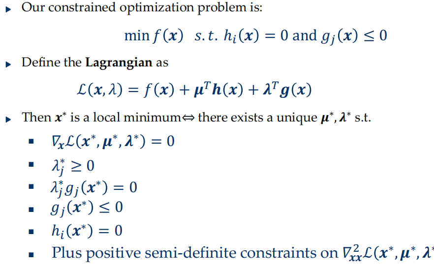
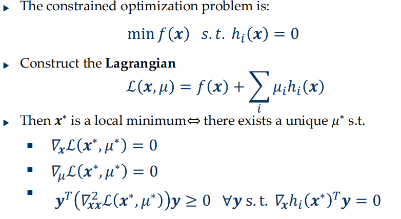
8. Lagrange Multipliers and the Karush-Kuhn-Tucker conditions

   • equality constraints
   
   • inequality constraints
   
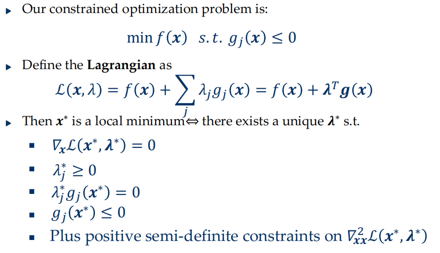
   • equality and inequality constraints
   

评论