13 Reinforcement Learning
Introduction
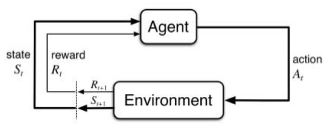
- agent: the learner and decision-maker
- environment: the thing agent interacts with, comprising everything outside the agent
- reward: special numerical values that the agent tries to maximize over time
- state and action: in general, actions can be any decisions we want to learn how to make, and the states can be anything we can know that might be useful in making them
-
最终要得到的是policy \(\pi\),输入是state或其他包括reward等的内容,输出为对应的action
-
data: (State, Action, Reward)
- An RL agent must learn by trial-and-error 反复试错,策略一初始化就要开始跑,算reward
-
Actions may affect not only the immediate reward but also subsequent rewards(Delayed effect) 一个行动会对长期许多步的reward都有影响
-
elements of RL
- policy: a map from state space to action space 可能是stochastic(随机)的
- reward function: map each state or state-action pair to a real number, called reward
- value function: value of a state or state-action pair is the total expected reward, starting from the state or state-action pair 从当前状态跑到正无穷或结束的总reward
Goal
-
maximize the Value function
-
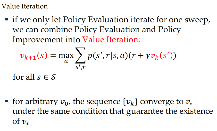
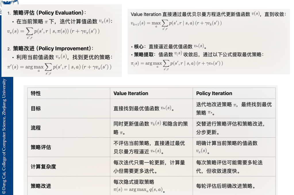
Value iteration and Policy iteration are two classic approached to this problem. But essentially both are dynamic programming.
-
Q-learning是最新的一个算法,是一种时序差分的方法
-
Algorithm
-
Goal
- policy \(\pi(a|s)\)
- reward hypothesis: maximization of the expected value of the cumulative sum of reward
-
Return
-
return G is the formally defined cumulative sum of reward
-
episodic task(回合式任务): episode means there are some special states, after which agent-environment interaction should restart or stop \(G_t = R_{t+1}+R_{t+2}+\cdots+R_T\), T is the time of final state
-
continuing task: the agent-environment interaction does not break naturally into identifiable episodes, but goes on continually without limit \(G_t=\sum_{k=0}^\infty\gamma^kR_{t+k+1},0\leq\gamma<1\), \(\gamma\) is called discount rate
-
unified Notation for Episodic and Continuing Tasks
\(G_t=\sum_{k=0}^\infty\gamma^kR_{t+k+1},0\leq\gamma\leq1\)
- if continuing tasks, \(\gamma\neq1\)
- if episodic task, adding an absorbing state after the final state(called terminal state) that transitions only to itself and that generates only zero reward, so we get \(R_{T+1}=R_{T+2}=\cdots=0\) 即final state之后的reward都视为0即可
- 但episodic也可以\(\gamma<1\)
-
-
Finite MDP
-
马尔可夫性
\[ Pr\{S_{t+1}=s',R_{t+1}=r|S_0,A_0,R_1,\dots,S_{t-1},A_{t-1},R_t,S_t,A_t\}=\newline Pr\{S_{t+1}=s',R_{t+1}=r|S_t,A_t\} \]-
MDP: 满足马尔可夫性的强化学习任务,状态空间和行为空间有限则为有限MDP
-
the dynamic of a finite MDP
\[ p(s',r|s,a)=Pr\{S_{t+1}=s',R_{t+1}=r|S_t=s,A_t=a\} \]-
从dynamic我们可以得到
-
the expected rewards for state–action pairs $$ r(s,a)=\mathbb{E}[R_{t+1}|S_t=s,A_t=a]=\sum_rr\sum_{s'}p(s',r|s,a) $$
-
state-transition probabilities $$ p(s'|s,a)=Pr{S_{t+1}=s'|S_t=s,A_t=a}=\sum_rp(s',r|s,a) $$
-
-
value function
-
the state-value function for policy \(\pi\),
\[ v_\pi(s)=\mathbb{E}_\pi[G_t|S_t=s]=\mathbb{E}_\pi[\sum_{k=1}^\infty R_{t+k+1}|S_t=s] \] -
the action-value function for policy \(\pi\),
\[ q_\pi(s,a)=\mathbb{E}_\pi[G_t|S_t=s,A_t=a]=\mathbb{E}_\pi[\sum_{k=1}^\infty\gamma^k R_{t+k+1}|S_t=s,A_t=a] \] -
如果没有dynamic,v和q不能互转
-
relation between the two value functions
\[ \begin{aligned} & v_{\pi}(s)=\mathbb{E}_{\pi}[q_{\pi}(s,A_{t})|S_{t}=s]=\sum_{a}\pi(a,s)q_{\pi}(s,a)\newline & q_{\pi}(s,a)=\mathbb{E}_{\pi}[R_{t+1}+\gamma v_{\pi}(S_{t+1})|S_{t}=s,A_{t}=a]\newline & =\sum_{s^{\prime},r}p(s^{\prime},r|s,a)(r+\gamma v_{\pi}(s^{\prime})) \end{aligned} \]
-
-
Bellman equation for \(v_\pi\)
-
for every state \(s\), we have the unique solution as follows
\[v_\pi(s)=\sum_a\pi(a,s)q_\pi(s,a)=\sum_a\pi(a,s)\sum_{s',r}p(s',r|s,a)(r+\gamma v_\pi(s'))\]
-
-
Optimal Value Functions
-
最优策略是存在的,记为\(\pi_*\),可能不止一个,他们share同样的state-value function,同时有以下:
\[ v_*(s)=\max_\pi v_\pi(s) \newline q_*(s,a)=\max_\pi q_\pi(s,a) \] -
最优策略在任何状态下都是最优的,不管MDP的初始状态如何
-
Bellman optimality equation
\[ v_*(s)=\max_aq_*(s,a)=\max_a\sum_{s',r}p(s',r|s,a)(r+\gamma v_*(s')) \]
-
-
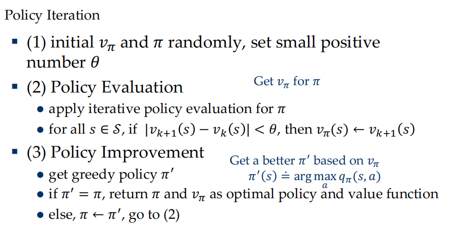
DP: 给定符合MDP的perfect model环境,使用DP可以计算得到optimal policies
-
策略评估,使用iterative policy evaluation,其中k为迭代次数 $$ v_{k+1}(s)=\sum_a\pi(a,s)\sum_{s^{\prime}r}p(s^{\prime},r|s,a)(r+\gamma v_k(s^{\prime})) $$
-
policy improvement theorem
-
deterministic policy: if policy \(\pi\) is deterministic then only one action has non-zero probability under any state \(s\), note that action \(\pi(s)\)
-
如果\(\pi\)和\(\pi'\)是一对deterministic policy,使得对所有s,\(q_\pi(s,\pi'(s))\geq v_\pi(s)\),则显然\(v_{\pi'}(s)\geq v_{\pi}(s)\)
-
proof
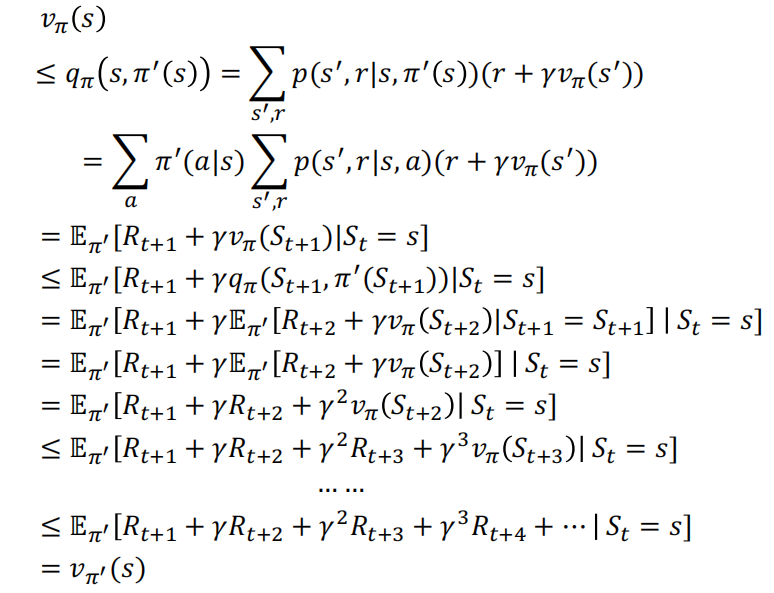
- 因此
$$ \begin{aligned} \pi^{\prime}(s) & =\arg\max_aq_\pi(s,a) \newline
& =\arg\max_{a}\sum_{s^{\prime},r}p(s^{\prime},r|s,a)\left[r+\gamma v_{\pi}(s^{\prime})\right] \end{aligned} $$ -
-
整体算法:
- 每次策略评估直到收敛,之后提取最优策略
-
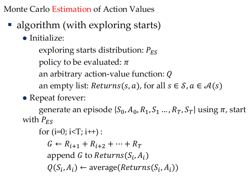
Monte Carlo Methods
-
treat the unknown as an expectation, and estimate it by sampling and averaging
-
sufficient exploration
- 需要得到无限的episodes
- exploring starts: the first state-action pair \((S_0,A_0)\) of each episode is sampled from a distribution that every state-action has a non-zero probability
当蒙特卡洛评估收敛时,我们可以进行一次策略提升。但是实际中训练难度很大
-
下一次策略评估时
-
若保留前一次的returns,由于之前的并不是由新策略生成的,因此会产生bias,同时很耗内存
-
但如果不保存,又需要很多次数来重新生成收敛的Q
-
constant-\(\alpha\) MC
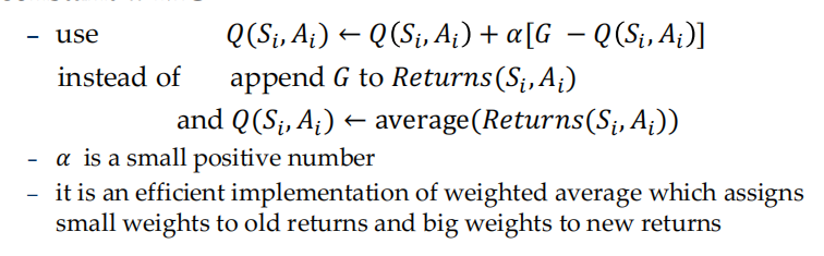
- 一般\(\alpha\)取0.1
-
TD Learning
update the value function when simulate only one step $$ V(S_t)\leftarrow V(S_t)+\alpha[R_{t+1}+\gamma V(S_{t+1})-V(S_t)] $$ 优点是快
- 对比DP,不需要环境模型
- 对比MC,online fashion上运行,对continuing task也适用
TD error $$ \delta_t\doteq R_{t+1}+\gamma V(S_{t+1})-V(S_t) $$
-
Sarsa
-
\(\epsilon\)-greedy
随尝试次数增加,\(\epsilon=\dfrac{1}{\sqrt{t}}\)减少
-
since \(p(s',r|s,a)\) is unclear, we have to estimate action-value \(Q\) rather than state-value \(V\)
-
algorithm
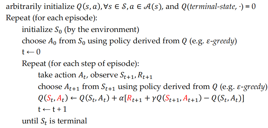
-
in Sarsa, \(Q(s,a)\) has theoretical guarantee for convergence
-
-
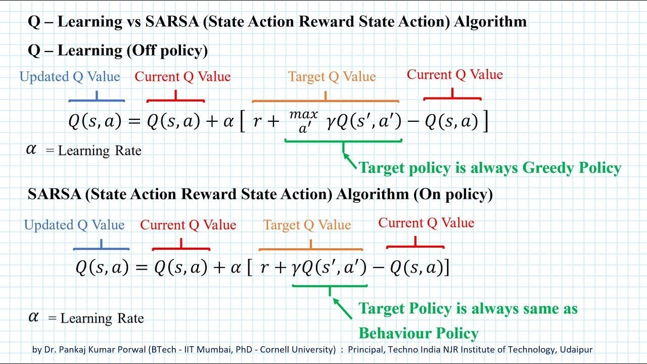
Q-learning
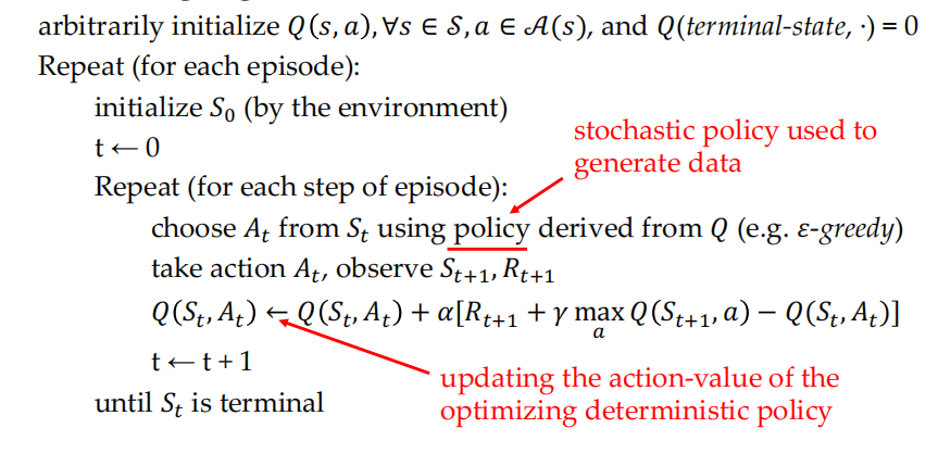
- on-policy and off-policy
- like Sarsa, if the policy to optimize is the same as the policy to generate training data, these control methods called on-policy
- like Q-learning, if the policy to optimize is different from the policy to generate training data, these control methods called off-policy
- on-policy and off-policy
- Double Q-Learning
- Essentially, we use one policy model for taking actions, and update it on-the-fly, while for the other value model, we use it to estimate the q-value for each action-state pair.
- The architecture for policy model and value model can be the same. In this case, we update the weight for value model with the weight of policy model several(say 500) iterations.
Exploration VS Exploitation
- Connected to: bias vs. variance, tradeoff.
-
Extremes: greedy vs. random acting
-
At the beginning of learning, we may want more exploration to know the environment
- As time goes by, we may want more exploitation
- Q-learning converges to optimal Q-values if
- Every state is visited infinitely often (due to exploration)
- The action selection becomes greedy as time approaches infinity
- The learning rate a is decreased fast enough but not too fast
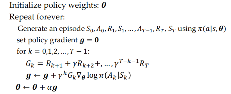
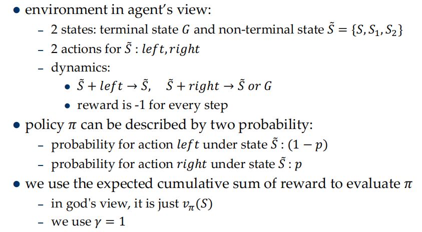
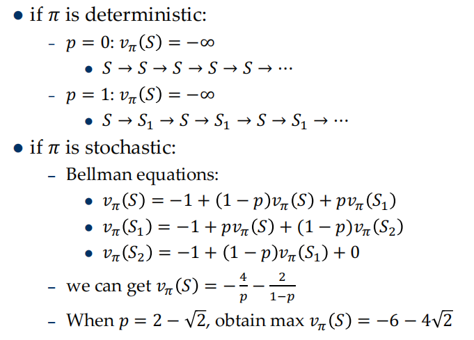
Policy Gradient Methods
in real world, we often can not get enough state information about the environment. At these time, the Markov property does not hold
the optimal policy may not be deterministic policy
example: Short corridor with switched actions
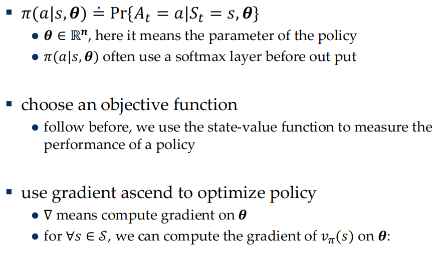
- REINFORCE