12 Dimensionality Reduction

• Linear Methods

  • Principal Component Analysis (PCA) unsupervised
  • Linear Discriminant Analysis (LDA) supervised
  • Locality Preserving Projections (LPP)
  • The framework of graph based dimensionality reduction.

• Non-linear Methods

  • Kernel Extensions for nonlinear algorithms.
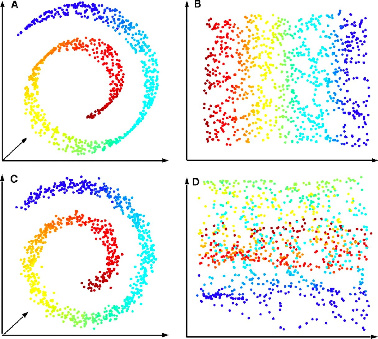
  • Manifold Learning
  • ISOMAP
  • Locally Linear Embedding
  • Laplacian Eigenmap

Principal Component Analysis

• The new variables, called principal components (PCs), are uncorrelated, and are ordered by the fraction of the total information each retains.

• main steps for computing PCs

  • Form the covariance matrix \(S=\frac{1}{n}\sum_{i=1}^n(x_i-\overline{x})(x_i-\overline{x})^T\).
  • Compute its eigenvectors: \(\{a_i\}^p_{i=1}\)
  • Use the first d eigenvectors \(\{a_i\}^d_{i=1}\) to form the d PCs.
  • The transformation A is given by \(A=[a_1,\dots,a_d]\)

• Pre-Processing of PCA

  • standardization: \(x'=\dfrac{x-\overline{x}}{\sigma}\)

• PCA的最优性质：PCA的projection在所有d规模的线性projection中最小化以下误差，即PCA保留了最多的信息。以下做的就是用A投影后再反投影回去得到重构的数据，比较和原数据的距离

  • X is centered data matrix

$$ \min_{A\in\mathcal{R}^{p\times d}}|X-AA^TX|_F^2 s.t. A^TA=I_d $$

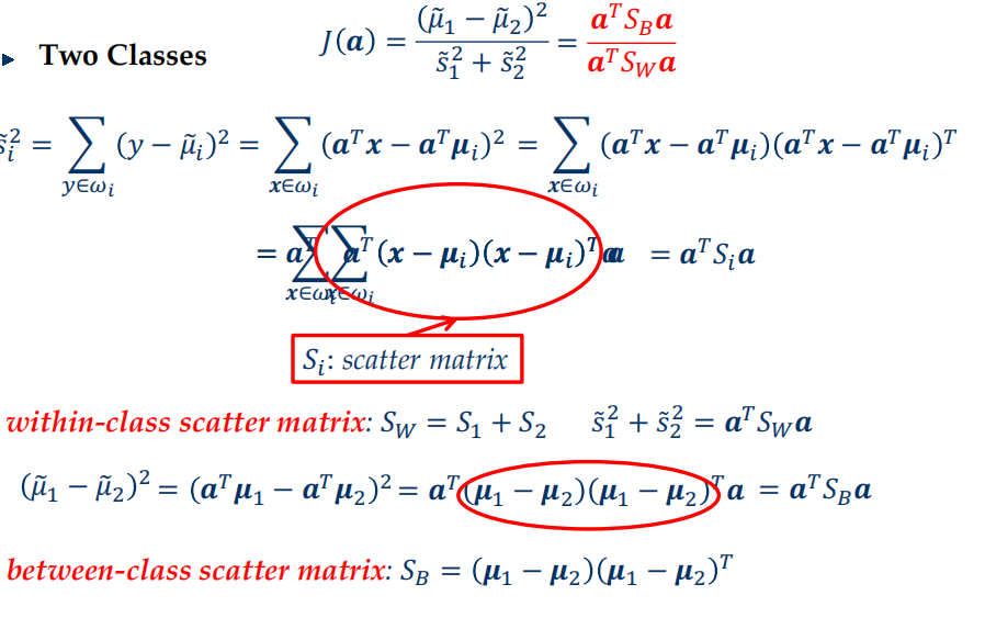
Linear Discriminant Analysis (Fisher Linear Discriminant)

• 最大化类间距离，最小化类内距离
• \(S_i\) 散度矩阵

• Main steps:

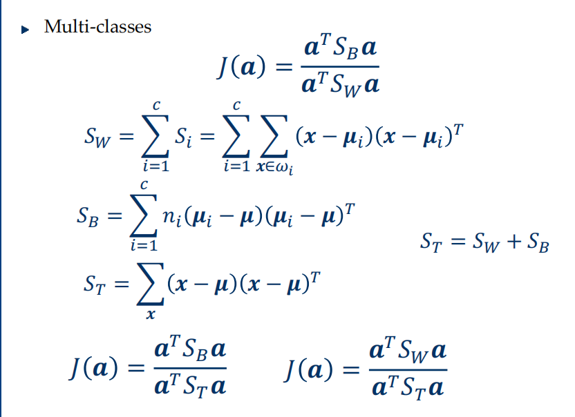
  • Form the scatter matrices \(S_B\) and \(S_W\)

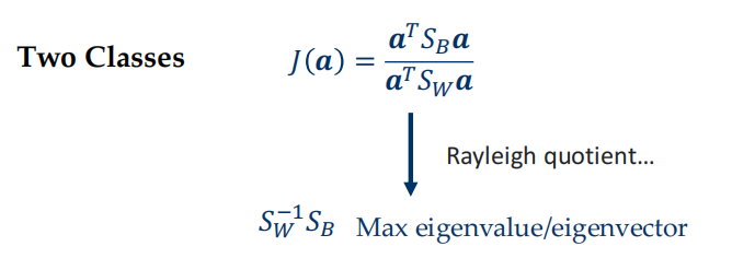
  • Compute the eigenvectors \(\{a_i\}_{i=1}^{c-1}\) corresponding to the non-zero eigenvalue of the generalized eigenproblem: $$ \begin{aligned} S_Ba &=\lambda S_Wa \newline &or \newline S_Ba&=\lambda S_T a \end{aligned} $$

  • The transformation A is given by \(A=[a_1,\dots,a_{c-1}]\)

Locality Preserving Projections (LPP)

不考

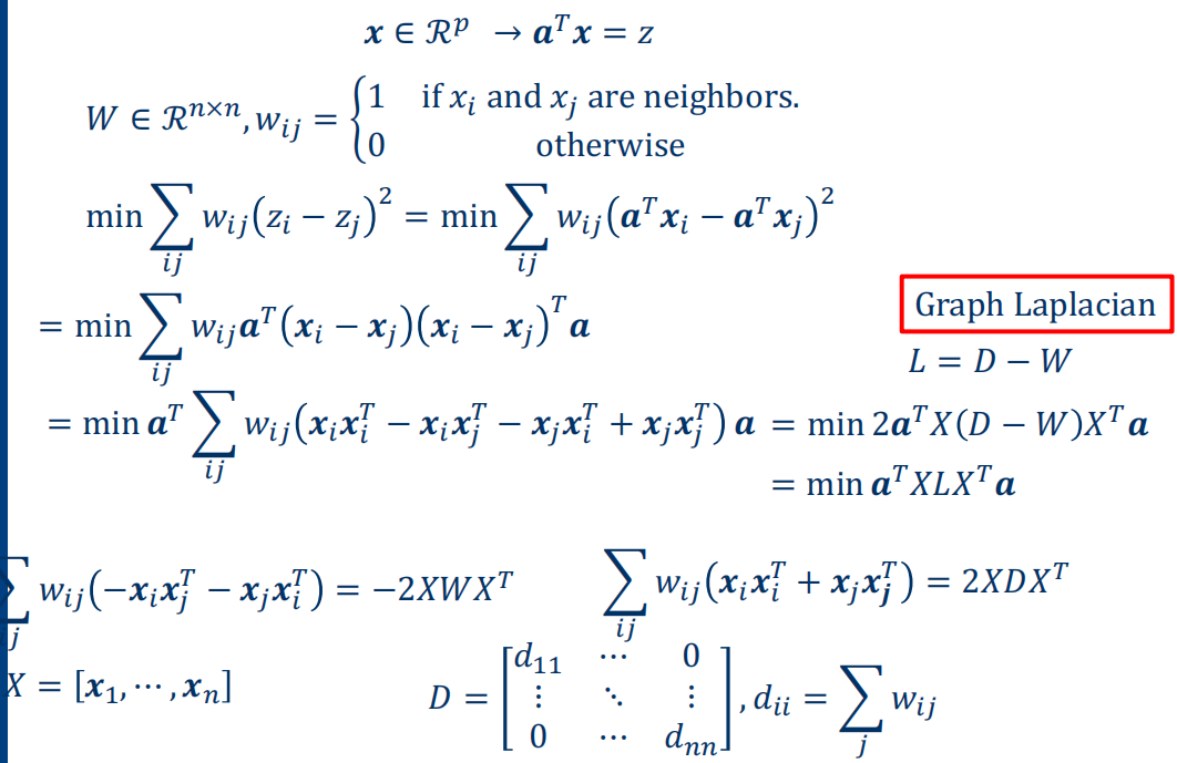
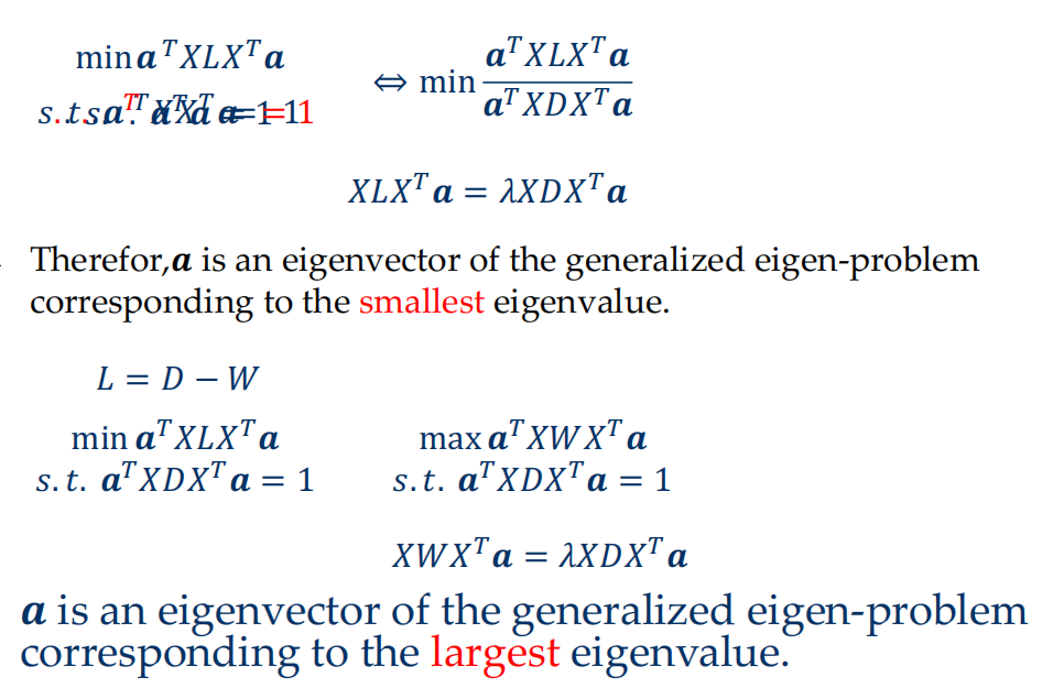
• LPP is equivalent to LDA when a specifically designed supervised graph is used
• LPP is similar to PCA when an inner product graph is used

Manifold Learning

Manifold

• In mathematics, a manifold is a topological space that locally resembles Euclidean space near each point
  • Each point has a neighborhood that is homeomorphic to the Euclidean space.
• a square and a circle are homeomorphic to each other, but a sphere and a torus are not.

Multi-Dimensional Scaling (MDS)

• 希望降维后空间数据之间的距离和原始空间尽可能一致
• 首先计算原来的数据点对应的pair-wise距离矩阵\(D=(d_{ij})\in\mathbb{R}^{n\times n}\)，尝试找到一个k维的表示，使得\(\|z_i-z_j\|=d_{ij}\)
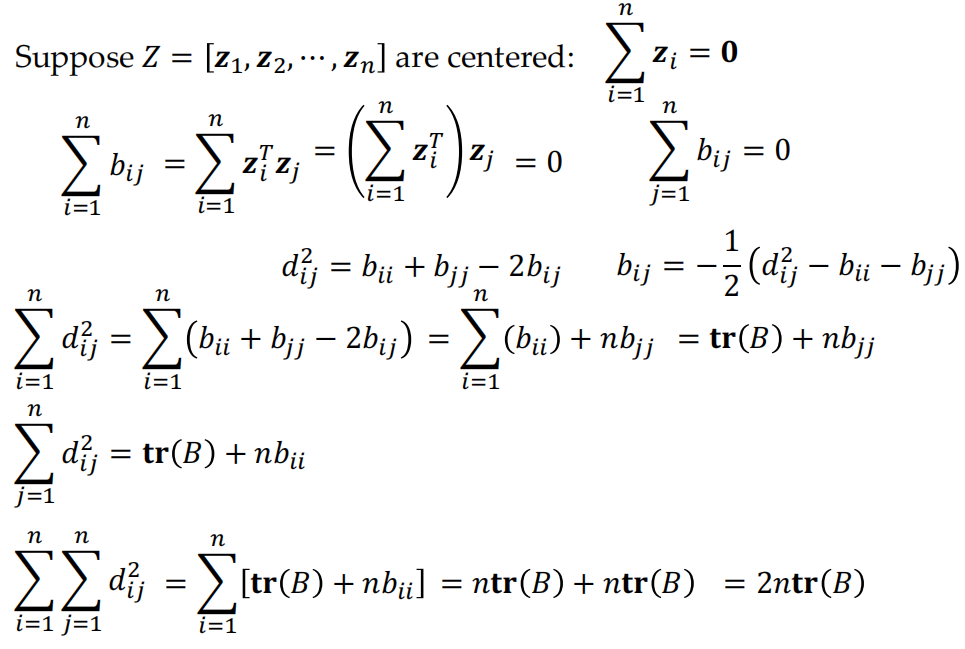
• suppose \(Z=[z_1,z_2,\dots,z_n]\), let \(B=Z^TZ\)
  • \(b_{ij}=z_i^Tz_j\)
  • \(d^2_{ij}=\|\mathbf{z}_i\|^2+\left\|\mathbf{z}_j\right\|^2-2z_i^Tz_j=b_{ii}+b_{jj}-2b_{ij}\)
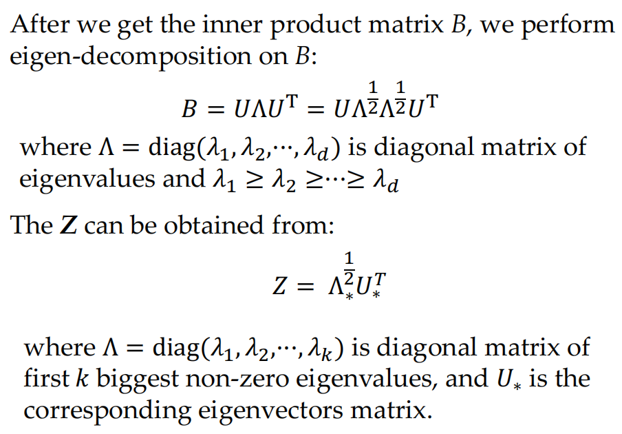
  • One possible Z can be obtained through eigen-decomposition of B
  • 假设Z的均值为0
  • main idea: D->B->Z
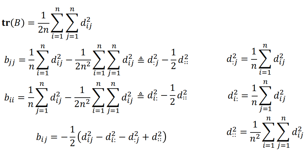
  • 通过一系列计算，我们可以得到矩阵B每个元素用D的表示，之后使用奇异值分解即可得到Z

• summarize:
  • Input: Distance matrix \(D\)
  • Algorithm:
    • compute \(d_{i:}^2=\frac1n\sum_{j=1}^{n}d_{ij}^2,d_{:j}^2=\frac1n\sum_{i=1}^{n}d_{ij}^2,d_{::}^2= \frac1{n^2}\sum_{i=1}^{n}\sum_{j=1}^{n}d_{ij}^2\)
    • compute inner product B \(b_{ij}=-\frac12(d_{ij}^2-d_{i:}^2-d_{:j}^2+d_{::}^2)\)
    • apply eigen-decomposition on \(B\)
    • Select first \(k\) biggest non-zero eigenvalues and corresponding eigenvectors, the target low-dimensional data matrix can be obtained from \(Z=\Lambda_{*}^{\frac12}U_{*}^{T}\)
  • Output: the k-dimensional data matrix \(Z\)

ISOMAP

• Step 1:

  • Define the graph G over all data points

  • Connect neighbor points and define the edge length equals to Euclidean distance

  • For point \(x_i\) and \(x_j\), if they are: - closer than \(\epsilon\) (\(\epsilon\)-ISOMAP) - \(x_i\) is one of the k nearest neighbors of \(x_j\) (k-ISOMAP)

• Step 2:

  • Compute shortest paths \(d(x_i,x_j)\) in G Floyd-Warshall or Dijkstra

• Step 3:

  • Apply MDS on \(d(x_i,x_j)\) to find lower-dimensional embedding

Locally Linear Embedding

• only focus on the local

• for a data point \(x\), and its neighbors \(x_1,x_2,\dots,x_k\), we assume \(x=w_1x_1+w_2x_2+\dots+w_kx_k\) ,and \(\sum w_i=1\)

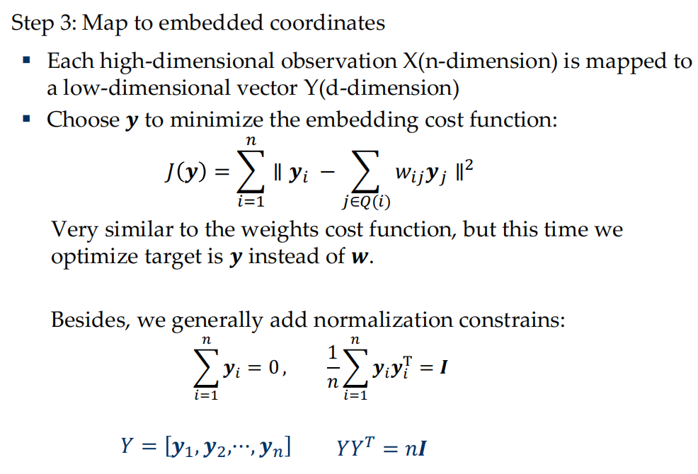
• and for projected data points \(y\), and its neighbors \(y_1, y_2, \dots, y_k\), we hope \(y\approx w_1y_1+w_2y_2+\cdots+w_ky_k\)

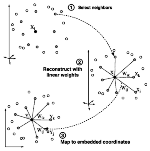
• Step 3

Other Interesting DR Algorithms

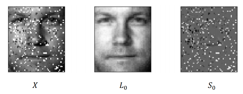
Robust PCA

1. suppose we have a high-dimension matrix \(X\): \(X=L_0+S_0\)

   • \(L_0\), meaningful part, low-rank
   • \(S_0\), noisy part, sparse
   

2. target:

   \[ \begin{aligned}minimize\ \ \ &rank(L)+\lambda\|S\|_0 \newline subject\ to\ \ \ &L+S=X\end{aligned} \]

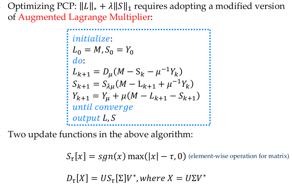
但是这个优化目标非凸且NP-hard，因此使用以下PCP(Principle Component Pursuit) surrogate error

$$ \begin{aligned} minimize\quad &|L|_*+\lambda|S|_1 \newline subject\quad to\quad &L+S=X \end{aligned} $$

• \(\|L\|_*\) is the nuclear norm, i.e. the sum of the singular values of L, will lead to low rank for L

• \(\|S\|_1\) will lead to sparsity for \(S\) like Lasso decay

3. Pros: The noise \(S_0\) can be arbitrarily large as long as it is sparse enough

4. constraints

   • The low-rank part \(L_0\) can not be sparse;
   • The sparse part \(S_0\) can not be low-rank.

AutoEncoder

1. An unsupervised neural network based framework for dimensionality reduction.
2. 利用反向传播算法使得输出值等于输入值的神经网络，它先将输入压缩成潜在空间表征，然后将这种压缩后的空间表征重构为输出。它的隐藏成层的向量具有降维的作用。
3. 训练
   1. 加入噪声尝试去噪
   2. Feature Disentanglement:获取embedding输出每一维分别对应什么信息

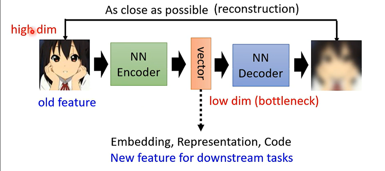
3. Embedding is using a low-dimensional vector to represent an “object”

Word2vec

1. A word’s meaning is given by the words that frequently appear close-by

2. context: When a word w appears in a text, its context is the set of words that appear nearby (within a fixed-size window).

3. Key ideas:

   • We have a large corpus of text

   • Every word in a fixed vocabulary is represented by a vector

   • Go through each position t in the text, which has a center word c and context (“outside”) words o

   • Use the similarity of the word vectors for c and o to calculate the probability of o given c (or vice versa)

   • Keep adjusting the word vectors to maximize this probability

4. two tasks

   • Skip-grams: predict context (”outside”) words (position independent) given center word
   • Continuous Bag of Words (CBOW): predict center word from (bag of) context words

5. objective function: loglikelihood

   \[ Likelihood=L(\theta)=\frac{1}{T}\prod_{t=1}^T\prod_{-m\leq j\leq m,j\neq0}P(w_{t+j}|w_t;\theta) \]

   • use two vectors per word w

   • \(v_w\) when w is a center word

   • \(u_w\) when w is a context(outside) word

   • then $$ P(o|c)=\frac{\exp(u_0^Tv_c)}{\sum_{w\in V}\exp(u_w^Tv_c)} $$

   • 提高效率, negative sampling

   \[ P(o|c)=\frac{\exp(u_0^Tv_c)}{\frac{|V|}{|V^{\prime}|}\Sigma_{w\in V^{\prime}}\exp(u_w^Tv_c)} \]
   • Or we can take the probability of each word into account

6. after training, we get outside embedding U and center embedding V for each word. Just average them or sum them to get the final embedding for each word.

评论