Lec.04: Model Fitting and Optimization

Optimization

1. objective function, inequality constraint functions, equality constraint functions $$ \begin{aligned}\text{minimize} & f_0(x)\newline \text{subject to} & f_i(x)\leq0,\quad i=1,\ldots,m\newline &g_i(x)=0,\quad i=1,\ldots,p\end{aligned} $$

   Example

   

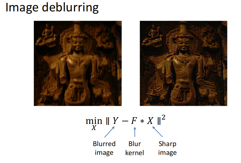
2. Model fitting: a mathematical model \(b=f_x(a)\)

3. MSE: \(\widehat{x}=\underset{x}{\operatorname*{argmin}}\Sigma_i(b_i-a_i^Tx)^2\)

   • Why MSE: 对噪声没有任何先验知识情况下，认为各种噪声的和是高斯噪声
   • Gaussian noise: \(b_i=a_i^Tx+n,n\sim G(0,\sigma)\)
   • then given \(x\), the likelihood of observing \((a_i,b_i)\) is

   $$ P[(a_i,b_i)|x]=P[b_i-a_i^Tx]\propto\exp-\frac{(b_i-a_i^Tx)^2}{2\sigma^2} $$

   • if the data points are independent

   $$ \begin{aligned} &\begin{aligned}P[(a_1,b_1)(a_2,b_2)...|x]\end{aligned} \newline &=\prod_{i}P[(a_{i},b_{i})|x] \newline &=\prod_iP[b_i-a_i^Tx] \newline &\propto\exp-\frac{\sum_{i}(b_{i}-a_{i}^{T}x)^{2}}{2\sigma^{2}}=\exp-\frac{|Ax-b|_{2}^{2}}{2\sigma^{2}} \end{aligned} $$

   • MLE = 最大化上述概率相当于最小化\(||Ax-b||^2_2\)。因此MSE = MLE with Gaussian noise assumption

Numerical methods

1. overall:

   • \(x\leftarrow x_0\%\) Initialization
   • while not converge
     • \(\boldsymbol{h}\leftarrow\)descending_direction\((\boldsymbol x)\ \%\) determine the direction
     • \(\alpha\leftarrow\)descending_step\((\boldsymbol{x},\boldsymbol{h})\ \%\) determine the step
     • \(x\leftarrow x+\alpha\boldsymbol{h}\ \%\) update the parameters

2. Taylor expansion

   • First-order: \(F(x_k+\Delta x)\approx F(x_k)+J_F\Delta x\),\(J_F=[\dfrac{\partial f}{\partial x_1}\cdots\dfrac{\partial f}{\partial x_n}]\)为Jacobian matrix
   • Second-order: \(F(x_k+\Delta x)\approx F(x_k)+J_F\Delta x+\dfrac{1}{2}\Delta x^TH_F\Delta x\),\(H_F\)为Hessian matrix

   $$ \mathbf{H}=\begin{bmatrix}\frac{\partial^2f}{\partial x_1^2}&\frac{\partial^2f}{\partial x_1\partial x_2}&\cdots&\frac{\partial^2f}{\partial x_1 \partial x_n}\newline \newline \frac{\partial^2f}{\partial x_2 \partial x_1}&\frac{\partial^2f}{\partial x_2^2}&\cdots&\frac{\partial^2f}{\partial x_2 \partial x_n}\newline \newline \vdots&\vdots&\ddots&\vdots\newline \newline \frac{\partial^2f}{\partial x_n \partial x_1}&\frac{\partial^2f}{\partial x_n \partial x_2}&\cdots&\frac{\partial^2f}{\partial x_n^2}\end{bmatrix} $$

3. Steepest descent method: When direction of \(\Delta x\) is same as \(-J_F^T\), the objective function descend steepest

   • Advantage
     • Easy to implement
     • Perform well when far from the minimum
   • Disadvantage
     • Converge slowly when near the minimum
     • Waste a lot of computation
   • Reason
     • Only use first-order derivative
     • Does not use curvature(曲率)

4. determine the step size

   • exact line search: too slow
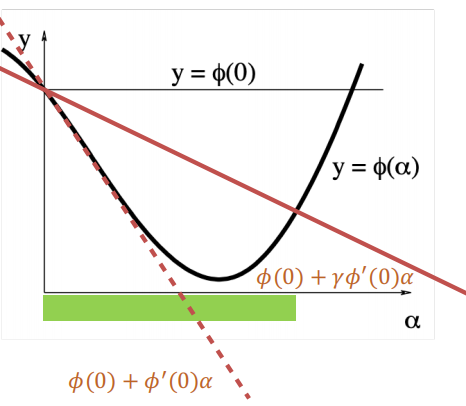
   • backtracking algorithm
     • initial \(\alpha\) with a big value
     • decrease \(\alpha\) until $\phi(\alpha)\leq\phi(0)+\gamma\phi^{\prime}(0)\alpha, 0<\gamma<1 $

1. Newton method: 用二阶泰勒展开，Newton step \(\Delta x=-H_F^{-1}J_F^T\)

   • Advantage: fast convergence near the minimum
   • Disadvantage: Hessian矩阵的计算消耗资源量大。改进：近似计算Hessian阵

2. Gauss-Newton method: useful for solving nonlinear least squares

   • \(\widehat{x}=\underset{x}{\operatorname*{argmin}}\|R(x)\|_2^2=F(x)\),\(R(x)\)为残差

   • instead of expanding \(F(x)\), we expand \(R(x)\)

   • \(J_R\) is the Jacobian of \(R(x)\)

   \[ \begin{aligned}\|R(x_{k}+\Delta x)\|_2^2 & \approx\|R(x_{k})+J_{R}\Delta x\|_2^2\quad\newline & =\|R(x_{k})\|_2^2+2R(x_{k})^{T}J_{R}\Delta x+\Delta x^{T}J_{R}^{T}J_{R}\Delta x\end{aligned} \]

   • 最优解满足: \(J_R^TJ_R\Delta x+J_R^TR(x_k)=0,\Delta x=-(J_R^TJ_R)^{-1}J_R^TR(x_k)\)

   • 优点：不用算Hessian阵, fast to converge

   • 缺点：若\(J_R^TJ_R\)为奇异的，即不满秩，特征值有可能为0，算法不稳定

3. Levenberg-Marquardt：\(\Delta x=-(J_R^TJ_R+\lambda I)^{-1}J_R^TR(x_k)\),对\(\lambda>0\)，\(J_R^TJ_R+\lambda I\)一定是正定的

   • Advantage:
     • Start quickly: \(\lambda\uparrow\)
     • Converge quickly: \(\lambda\downarrow\)
     • Do not degenerate: \(J_R^TJ_R+\lambda I\) is always positive-definite
     • LM = Gradient descent + Gauss-Newton
     • \(\lambda\)很大 stepsize很小的gradient descent
     • \(\lambda\)很大 Guass-Newton

Robust estimation

1. Inlier: obey the model assumption

Outlier: differ significantly from the assumption

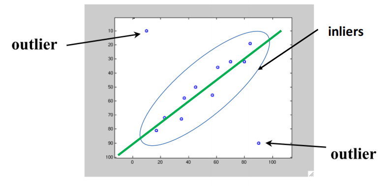
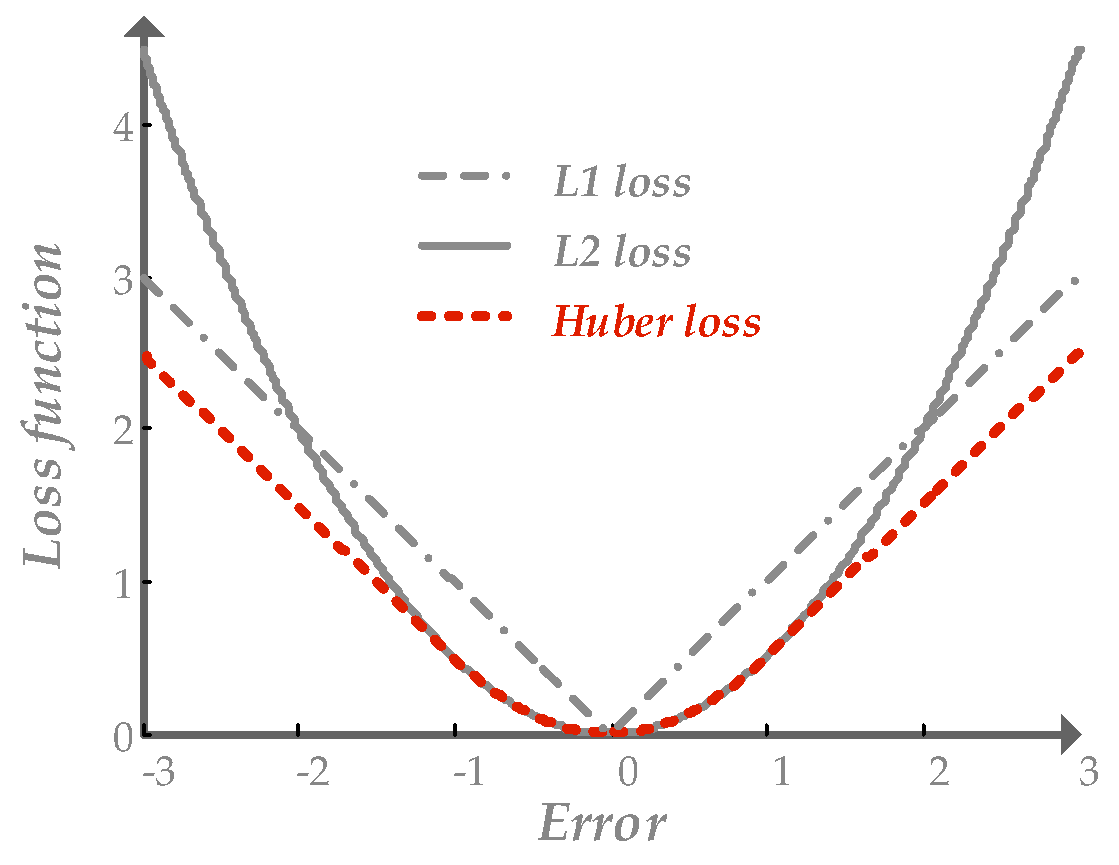
2. use other loss functions to replace MSE to reduce the effect
   • like L1, Huber. They are called robust functions

3. RANSAC(Random Sample Concensus): The most powerful method to handle outliers

   • Key idea: The distribution of inliers is similar while outliers differ a lot, use data point pairs to vote

4. ill-posed problem: the solution is not unique.

   • example:方程个数少于变量个数
   • solution: use prior knowledge to add more constraints
     • L2, L1 regularization

Graphcut

以后讲，不考

1. Image labeling problems

   • Assign a label to each image pixel
   • Neighboring pixels tend to take the same label
   • treat images as graphs
     • a vertex for each pixel
     • an edge between each pair

2. Measuring affinity: let \(i\) and \(j\) be two pixels whose features are \(f_i\) and \(f_j\) (color for example)

   • pixel dissimilarity
   \[ S\left(\mathbf{f}_{i},\mathbf{f}_{j}\right)=\sqrt{\left(\sum_{k}\left(f_{ik}-f_{jk}\right)^{2}\right)} \]
   • pixel affinity
   \[ w(i,j)=A\left(\mathbf{f}_{i},\mathbf{f}_{j}\right)=e^{\left\{\frac{-1}{2\sigma^{2}}S\left(\mathbf{f}_{t},\mathbf{f}_{j}\right)\right\}} \]

3. Graph cut

   • cut \(C=(V_A, V_B)\) is a partition of vertices \(V\) of a graph \(G\) into two disjoint subsets \(V_A\) and \(V_B\)
   • qcost of cut: sum of weights of cut-set edges \(cut(V_A, V_B)=\sum\limits_{u\in V_A,v\in V_B}w(u,v)\)

4. Segmentation as graph cut

   • Vertices within a subgraph have high affinity
   • Vertices from two different subgraphs have low affinity

5. normalized cut $$ \begin{aligned}\mathrm{NCut}\left(V_A,V_B\right)&=\frac{\operatorname{cut}\left(V_A,V_B\right)}{\operatorname{assoc}\left(V_A,V\right)}+\frac{\operatorname{cut}\left(V_A,V_B\right)}{\operatorname{assoc}\left(V_B,V\right)}\newline &\operatorname{assoc}(V_A,V)=\sum_{u\in V_A,v\in V}w(u,v)\end{aligned} $$

评论